Greeks and implied volatility are measures used by options traders to quantify risk. While rolling out our options products alpha, we received many requests to expose these in an API. After much research and hard work, we are excited to present, among other products, our new Options Snapshot API, which calculates Greeks and implied volatility on demand for a given contract.
In this article we will discuss four of the most commonly used Greeks: delta, gamma, theta, and vega, as well as some preliminary exposition on (implied) volatility and the Black-Scholes model. If you're educated on these topics already and don't need a refresher, you can instead read about how we chose and implemented a pricing model in the next section.
Definitions
Broadly speaking, the Greeks measure sensitivity of an option's fair price with respect to various parameters. Variations in the price of an option depend largely upon time, price of the underlying, and volatility. The Greeks are used to measure how the option's price varies with these quantities.
Black-Scholes model
Not to be confused with the Black-Scholes pricing formulas, the Black-Scholes model (also known as the Black-Scholes-Merton model) is a partial differential equation that expresses the fair value of a derivative asset (e.g., an option) given the price and volatility of the underlying stock, as well as the Greeks, which appear as partial derivatives in the equation.
The Black-Scholes model will be the basis for the rest of this article. But it is important to note that several critical assumptions are required for the model to hold:
- A risk-free asset exists, and it earns the risk-free interest rate;
- Assets can be bought and sold fractionally as well as sold short;
- There are no transaction costs;
- There are no arbitrage opportunities;
- Asset prices follow a log-normal distribution with constant drift and volatility. (In other words, the distribution of log-returns after a constant interval of time forms a "bell curve," or normal distribution.)
In the real world every one of these assumptions is violated at least to a small degree. However, the biggest culprit is assumption #5, which has long been known to be inaccurate and, as we will later see, is outright contradicted by observed market prices for options.
Despite its shortcomings, the Black-Scholes model is still regarded as a useful tool, if used appropriately. The resulting pricing equations are used to convert market prices of options into implied volatilities, which can be fed into yet more sophisticated models for calibration. Which is to say, in spite of the flaws in Black-Scholes, it still forms a robust basis for extension by other models.
Volatility
Volatility is, roughly speaking, the variability in the underlying asset's (the stock's) returns. It can be measured by calculating the standard deviation of log returns, and it is expressed as a percentage. A greater volatility implies greater variation in the returns of the underlying asset. Volatility raises the premium for an option, since there is a greater chance that the underlying asset will move favorably.
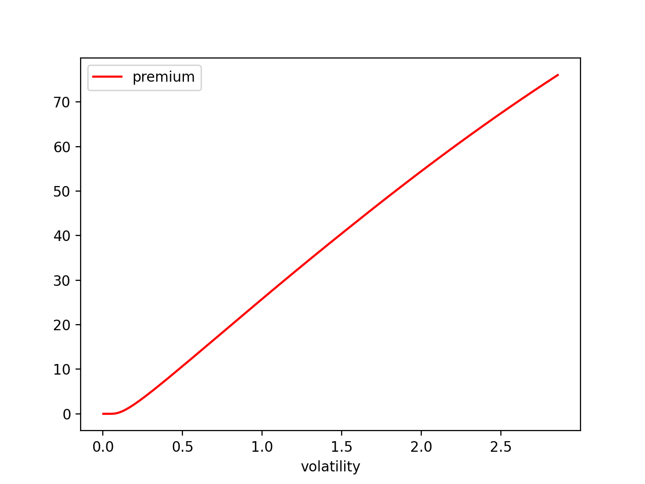
The above graph is the valuation of an option according to the Black-Scholes model. As discussed, the Black-Scholes model doesn't describe the real world accurately, but studying it is instructive when trying to reason about the dynamics of pricing derivatives.
As we can see in the very simple graph above, volatility and premium are almost linearly related. The higher the volatility, the greater premium demanded for the option. Note that other factors such as the spot price (price of the underlying stock), interest rates, and the passage of time can affect this curve. For example, if the time to maturity was instead 30 days, the chart would look like this:
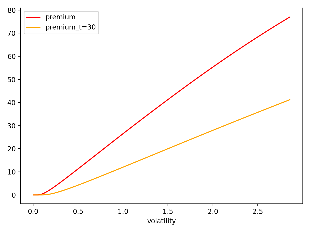
With only 30 days left to expiry and our contract still out of the money, our call option has less of a chance of expiring in the money. Hence, with volatility remaining the same, the shorter-dated contract has less value.
Implied Volatility
The Black-Scholes model assumes that you can characterize the movement patterns of an asset's price in terms of the volatility and drift alone, and the B.S. (Black-Scholes) equations do not depend on the drift at all. Hence, knowing the underlying price and the volatility should be sufficient to price an option (taking interest rates and dividends into account as appropriate). Volatility can be estimated by looking at historical data. However, if you try to calculate the "correct" valuation of an option using B.S. and using historical volatility as an estimator for the actual volatility, it will fail to reproduce market prices. In particular, the predicted price will (usually) fall below observed market prices. Why is that?
It turns out that Black-Scholes, by virtue of characterizing assets by volatility alone, underestimates risk in the underlying asset, and therefore underestimates risk in the derivative asset as well. More sophisticated volatility models attempt to measure this risk by factoring in discrete jumps and/or uncertainty in the future volatility. The value of volatility consistent with observed market prices under the Black-Scholes model is called the implied volatility.
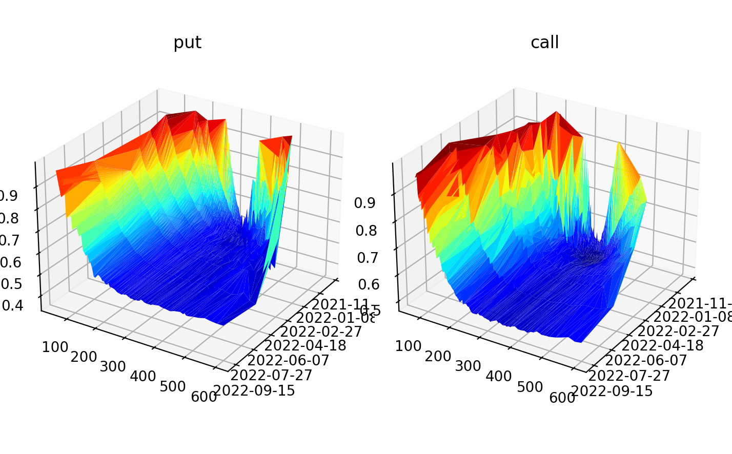
While volatility can be said to be a property of the underlying asset, implied volatility depends on the parameters of the option contract, particularly the expiration date and the strike price. This gives rise to an implied volatility surface, where implied volatility varies with respect to time to maturity and strike price:
As a simpler case, one can fix the expiration date and plot implied volatility against strike price alone, which creates what is variously referred to as a volatility smile or smirk, depending on the observed pattern. In this case, and generally for equity options, there is a smirk:
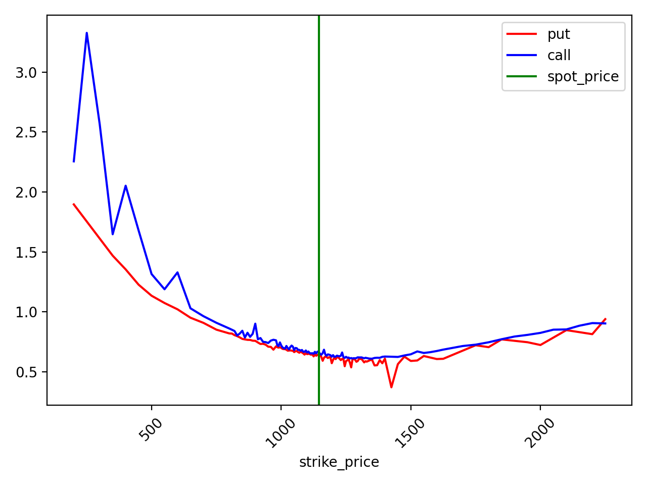
Volatility smiles were not observed until after the crash of 1987. Before then, implied volatilities were constant with respect to strike price, which is what the Black-Scholes model predicts. The existence of volatility smiles can be seen as evidence against the Black-Scholes model. As is often quoted from Riccardo Rebonato, implied volatility is "the wrong number to put in the wrong formula to get the right price." Despite this, the concept is so commonplace that traders sometime quote option prices in terms of implied volatility!
Delta
Delta (Δ) measures the sensitivity of the option's premium with respect to that of the underlying asset. For example, with a delta of 0.5 and all else being held equal, a $1.00 change in the underlying price approximately nets a $0.50 change in the option's premium. For call and put options, delta is positive and negative, respectively, because increases and decreases in the spot price are favorable for calls and puts, respectively.
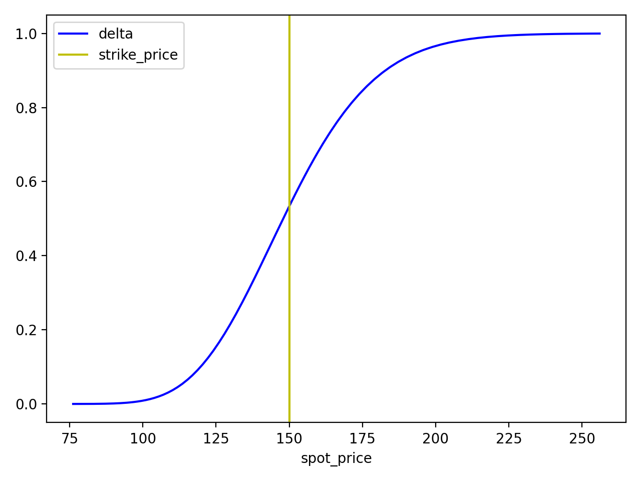
A strategy used in options trading is delta hedging, where an investor constructs a delta neutral portfolio -- that is, a portfolio whose total delta is zero. A simple example of a delta neutral portfolio is one with Δ shares sold short for each option contract in a long position. (In reality, most option contracts represent 100 shares in the underlying security, so you would actually need 100 times Δ shares sold short.)
Because delta is constantly changing (as are the other Greeks), delta-hedged portfolios are typically rebalanced on a daily basis – that is, re-allocated using the newest value of delta. For highly volatile assets, though, it might be necessary to rebalance even more frequently. Note that rebalancing incurs transaction costs, and so rebalancing can only be done so often before it begins to erode profits.
Gamma
Gamma (Γ) measures delta's sensitivity with respect to the price of the underlying. Because gamma measures change in delta, which in turn measures change of the option's premium, gamma is referred to as a second order Greek. For example, if gamma is 0.01, a $1.00 change in the underlying price would approximately net a 0.01 change in delta. Gamma is highest at the money, which is to say that delta changes quickly at the money. It is even higher for at-the-money options near expiry.
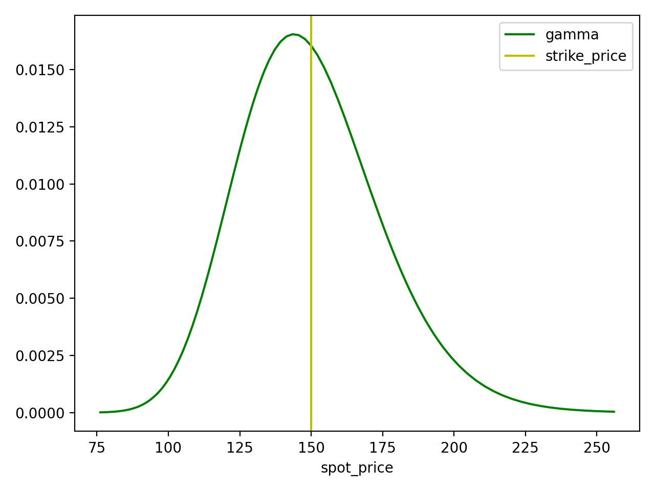
As with delta hedging, it is also possible to construct a gamma neutral portfolio, a strategy called delta-gamma hedging. If gamma is high enough, a delta neutral portfolio may still be at risk from movements in the underlying price, since delta may change and the portfolio may require rebalancing with respect to the new value of delta. Delta-gamma hedging also provides protection against larger price movements in the underlying, as delta remains closer to zero for a wider range of prices.
Theta
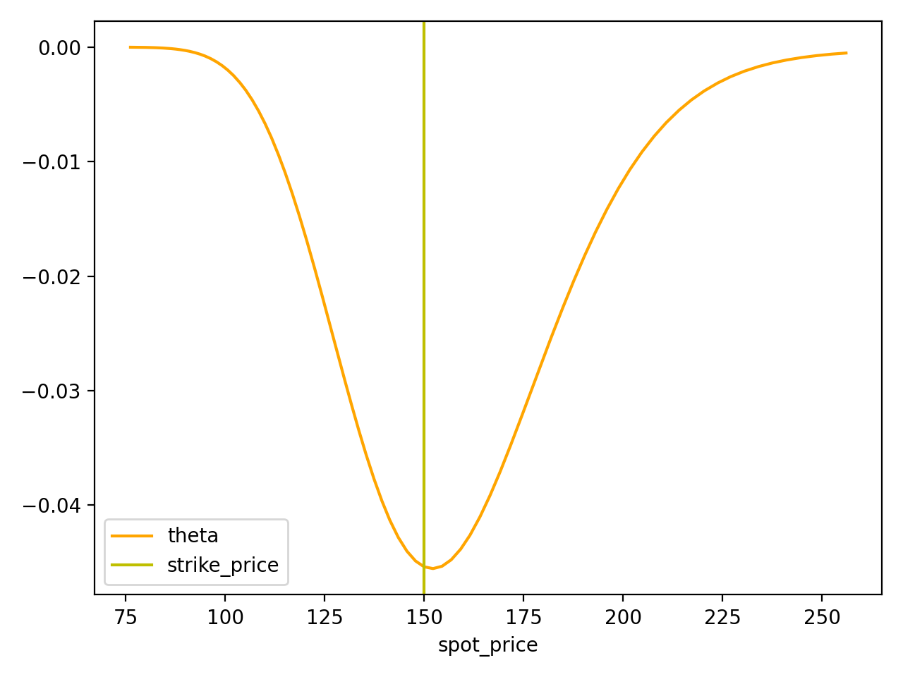
Theta (Θ) measures the sensitivity of the option's premium with respect to time. To be precise, it measures the expected change in premium after one day, all else being held equal (including but not limited to underlying price and volatility). For example, a theta of -0.02 means that after one day the option, with all else remaining equal, will be worth $0.02 less than the previous day. Theta is almost always negative for options, because a greater time to maturity generally presents a greater chance for profit. (In-the-money European options sometimes violate this rule, particularly on calls in the presence of high interest rates, and puts on dividend paying stocks, since they cannot be exercised early.)
Vega
Vega measures the sensitivity of the option's premium with respect to volatility. If vega is 0.6, then a 1% increase in volatility approximately nets a $0.60 change in the option's premium. Because volatility raises the premium for an option, vega is always positive.
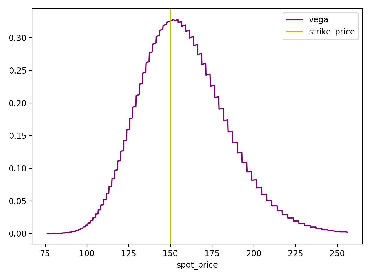
(Unlike the other Greeks, the model we chose doesn't provide convenient estimates for vega, so we have to resort to finite differences. The choppiness in the plot is probably an artifact of this method.)
Implementation
We chose the binomial options pricing model as it is straightforward, is reasonably fast, and is accurate for a variety of option styles. (Specifically, we chose the original Cox-Ross-Rubinstein variant.) Implementations as well as pseudocode are available on the internet. We found good explanations of the BOPM as well as some estimates for Greeks in Options, Futures, and Other Derivatives by John C. Hull, a classic introductory book for anyone interested in quantitative finance.
Collecting all of the necessary data together was time-consuming. The BOPM requires six inputs, which we will discuss below.
- Time to maturity
- Spot price
- Strike price
- Volatility
- Dividend yield
- Risk-free interest rate
As presented, the binomial options pricing model actually predicts the option premium given the volatility, not the other way around. However, since we are interested in computing implied volatility from option premium, we invert the model. This can be done by using a root-finding algorithm – while Newton's method is a typical choice, it requires us to compute the derivative of the function of interest. Instead we chose Brent's method, an algorithm that combines characteristics of the secant and bisection algorithms. It only requires two points at which the function takes opposite signs – at least one root will exists between those two points.
Implied volatility calculations are often done using the midpoint between the bid and ask for an option contract. This is because the options market has quite a low volume of trades (around 300/sec at the time of this post). On the other hand, there is a great deal of activity if you observe quotes on options contracts. Whereas the last trade for a contract may have been months ago, typically the most recent quote will have been within the last day. (As explained later, this is not a perfect solution.)
Calculating dividend yield
We use historical dividend payouts over the past year to estimate annualized yield. Another method is to simply use the most recent dividend and multiply by the frequency. There are more sophisticated methods of predicting dividend yield, however, and this is a direction we'd like to explore in the future.
In our calculations we use a continuous dividend yield, i.e. the stock pays out at a continuously compounded rate. However, for greater accuracy, the binomial options pricing model can easily accommodate discrete dividends, provided that one knows what dividends are being paid out during the option's lifetime.
Risk-free interest rate
The risk-free interest rate is the hypothetical rate of return on a "risk-free" investment. Together with no-arbitrage conditions, the existence of a risk-free asset is a core assumption of many financial models. One can derive the Black-Scholes partial differential equation by constructing a delta neutral portfolio and arguing that its rate of return must be the risk-free interest rate.
Typically treasury bond yields are used to estimate the risk-free interest rate -- however, options traders prefer to use something called SOFR, the Secured Overnight Financing Rate. Traders also use LIBOR -- the London Inter-Bank Offered Rate -- but in recent years SOFR has been recommended as the preferred alternative. You can read more on the transition for LIBOR to SOFR in this article from the SEC.
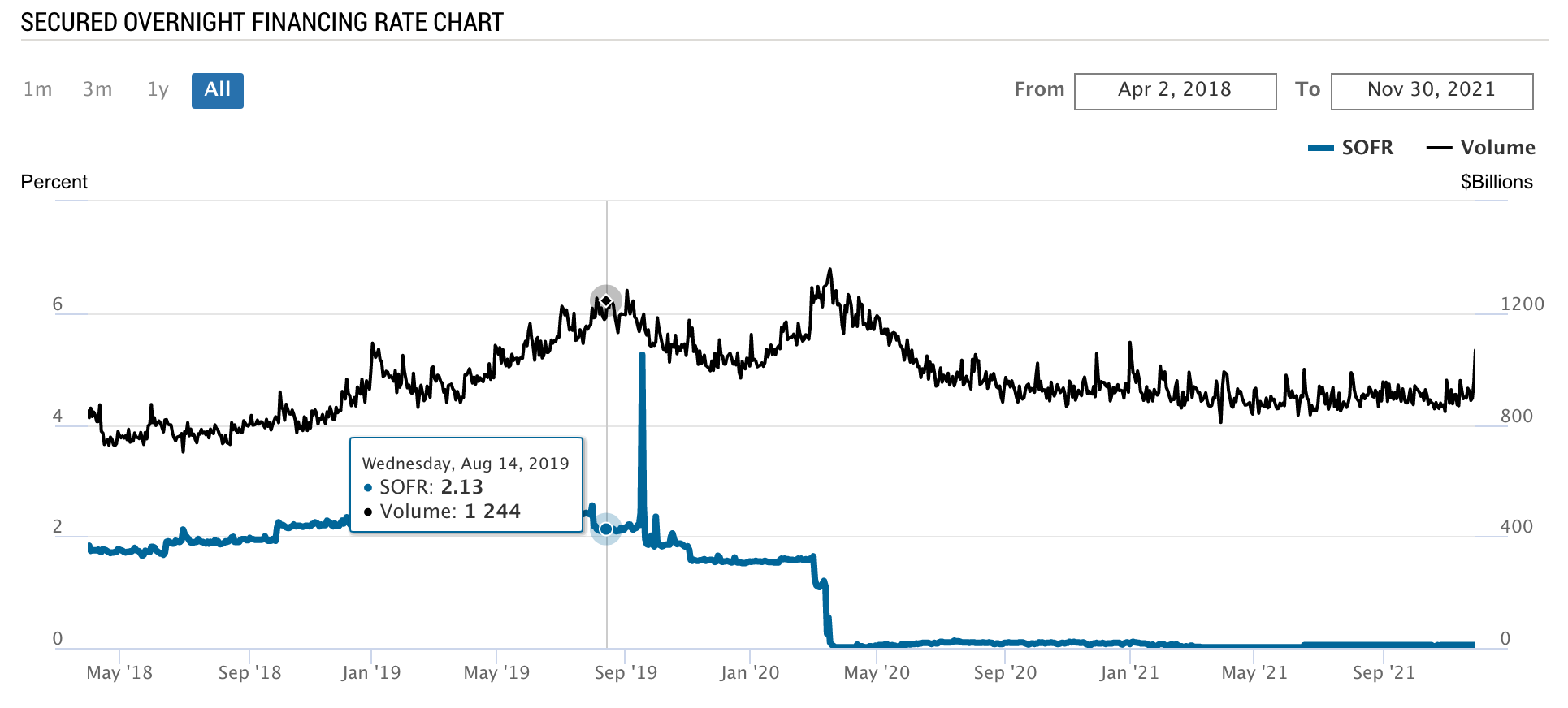
In March 2020, when COVID lockdowns began around the world, the Federal Reserve dropped interest rates near zero. We can see this reflected in the above graph. Before the pandemic, we can see that interest rates normally hovered around 2 percent.
Testing
When everything was said and done, we began running tests on some random contracts. We noticed that between 10-15% of contracts cause our model to fail, as their market prices violated no-arbitrage bounds on an option's premium. Briefly, for in-the-money options the premium should never fall below the intrinsic (exercise) value, otherwise this would represent an arbitrage opportunity. (For out-of-the-money options the intrinsic value is zero, so this never happens.) For example, suppose a trader is buying one contract of TSLA211203C01020000: that is, a call on TSLA expiring on Dec 3 2021 with a strike price of $1020 per share. (See How To Read A Stock Options Ticker.) If the spot price for TSLA were $1140 and they were able to buy a contract at $100 per share, they could profit instantly by exercising, buying at the strike price of $1020 and selling at $1140, pocketing $120 per share and a net profit of $20 per share. This constitutes arbitrage, something our pricing model assumes doesn't exist in the real world.
This reflects the difficulty of using the bid/ask midpoint as the input price. For in-the-money options, we observed a significant portion of contracts with bids that were below the intrinsic value. As in the above case, if someone were to actually sell to the buyer at such low bids, the buyer would be able to make money immediately by exercising. In a significant percent of cases this causes the midpoint to also fall below the intrinsic value, yielding an invalid input to our pricing model.
Conclusion
Researching and implementing a pricing model to compute implied volatility and Greeks taught us a lot about the options market. If you are just beginning to learn about options, we hope that the knowledge we gained will help you get started understanding how options -- and, more generally, derivatives -- are used. On the other hand, if you are a more advanced user of options data, hopefully we can provide some transparency into how our data is computed and what that means for your use case. In any case, we look forward to sharing our experiences as we continue to add more quantitative measures to our product stack.
